MAT 259 W06 Visualizing Information
Professor George Legrady
Experiments in Visualizing Machine Learning Algorithms
based on implementations of a neural network and the Kohonen self-organizing map
Experiments in Visualizing Machine Learning Algorithms
based on implementations of a neural network and the Kohonen self-organizing map
Visualization of a backpropogation neural network (BPNN) learning to play 5x5 Tic-Tac-Toe
Inspired by the course work for my Machine Learning course (with Professor Su) I created a visualization of a the process of training a BPNN. The final project for CS192B was to design a BPNN that learned to play a version of Tic-Tac-Toe. After a few failed attempts, I managed to build a BPNN that successfully made "correct" moves the majority of the time. Although my BPNN could not beat a thoughtful human player, it was undefeated when performing against other student's BPNN designs.
The general steps to training a BPNN are as follows:
0) Initialize the BPNN
A BPNN has a certain number of input nodes, hidden layer nodes, and output layer nodes. Each node is initialized with an activation weight, and each link between the nodes is initialized with a weight. I randomally initialized each of these with a number between -0.5 and +0.5.
1) Train the BPNN with a vector of inputs
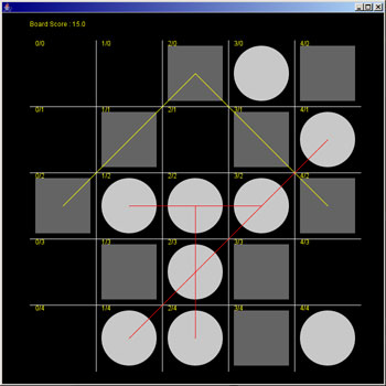
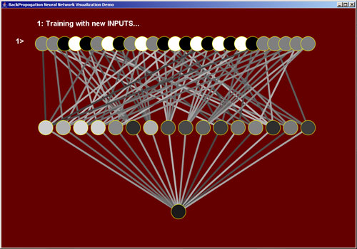
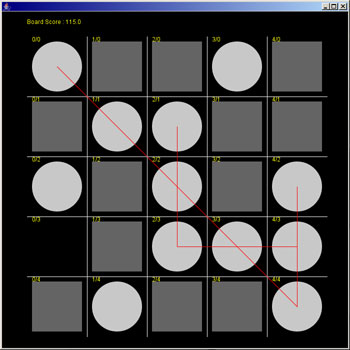
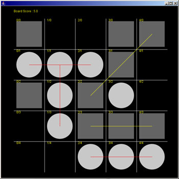
I wrote a program that calculated random legal positions of a 5x5 Tic Tac Toe board. I created 25 input nodes-- one for each space on the board. I assigned a value of +1.0 for an 'O', -1.0 for an 'X', and 0.0 if the space was empty. Additonally, I stored the expected value of this board position. I assigned a range of -1.0 to +1.0 depending on how good the board position was for 'O'.
2) Update the hidden layer of nodes
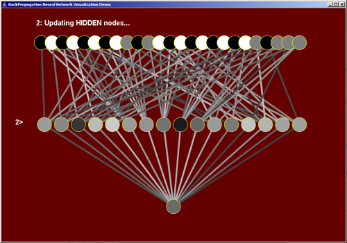
Each node in the hidden layer is updated by summing the multiple of each link weight times the activation weight of the input node. The activation weight of the hidden node is then calculated by retrieving the ouptut of a sigmoid function from that summation. I used the tanh function which returns a value between -1.0 and +1.0.
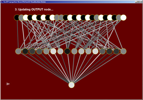
3) Update the output nodes
There is only one output node, and its activation is calculated in the same manner as a hidden node, except using the links from all of the hidden nodes to the one output node.
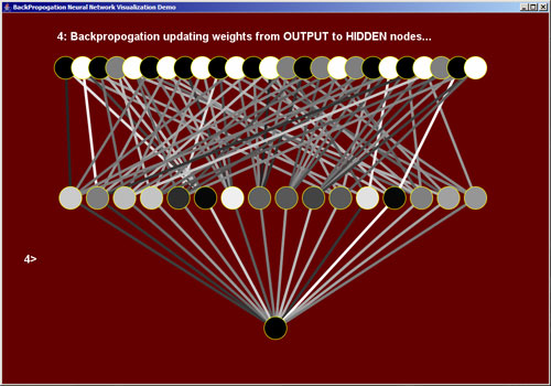
4) Update the links from the output nodes to the hidden nodes
Using the expected output which we calculated before passing in the input vector (step 1), we 'supervise' the training of the BPNN. This is done by finding the difference between the expected target output and the actual output activation, then "propogating" the derivative of the sigmoid function multiplied by that error backwards through the BPNN, updating the weights of the links accordingly.
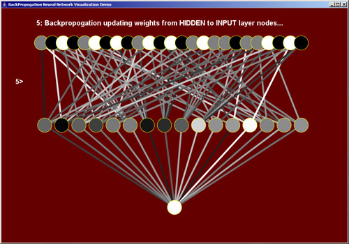
5) Update the links from the hidden nodes to the input nodes
We follow the exact same method when updating the weights of the links from the hidden nodes to the input nodes.
Steps 1 - 5 are repeated until the network is trained. I tested the training of the network by inputing random board positions to see if the output of the BPNN matched the calculated output as measured by my trajectory scoring program.
Because BPNNs are often considered 'black boxes', and because my first attempts at designing a BPNN returned random results, I wanted to build a visualization of the BPNN as it was trained so that I could better understand the process.
The following java program is an executable .jar file which can be downloaded and executed simply by double clicking on it, or by typing 'java -jar Bpnn.jar'
My final design linked each input node to two or three hidden nodes. Each input node represented a space on the board. Each hidden node represented a possible scoring trajectory. For instance, the first input node represented the top right corner of the board. Since that piece could possible effect the scoring of the board in three ways, it was linked to three hidden nodes. These hidden nodes represented the top-most row trajectory, the left-most column trajectory, and the top-left to bottom-right diagonal trajectory.
Visualization of a Kohonen Self-Organizing Map (SOM) learning to cluster and match colors
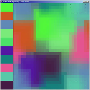
Another popular machine learning technique is the Self-Organizing Map (SOM), also called Kohonen maps after their inventor. In contrast to the BPNN described above, a SOM is an "unsupervised" learning alogrithm in that no target values need to by supplied in order to train the input data. I created a Java implementation of the basic SOM alogrithm so that I could visualize the step-by-step process of training a map. In this example, I train a 3-dimensional input vector on top of a 2-dimensional Kohonen map. I assign each attribute from an RGB color to a dimension of the input node. That is, the weight-space or attribute-space of the SOM has 3 dimensions, but the layout-space or view-space has 2-dimensions. A future project is to create 3-dimensional layouts.
0) Initialize the SOM
Like a BPNN, a SOM is initialized with a number of parameters, including the number of rows and columns, the topology, the learning rate, the neighborhood function, and the radius that the neighborhood function effects. For this demonstration I defined a 30x30 grid for the lattice, a learning rate of .3, and a radius of 10. I used a simple step function to define the updates for the nodes in the surrounding neighborhood. I emulated the topology of a torus by having the top and bottom of the grid wrap around, and likewise made the left and right sides wrap. The larger blocks of color on the left represent the input vector of colors.
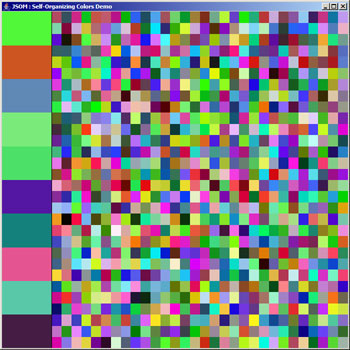 initialized random SOM
Each node in the SOM has its 3 weights set between 0 and 255, the range of values for each attribute in the RGB color model.
1) Randomally grab a member of the training data and find the best matching node to it inside the SOM
The colors in the input vector are chosen at random. The algorithm works by grabbing one of these input vectors (in this case, a color) at random. It compares itself to every node inside the SOM. The comparison method is simply the Euclidian distance formula. Once the best matching node is found, the node changes all of its weights to that of the input vector.
2) Iterate through the neighbors of this node and update their weights
The node then updates the weights of its surrounding nodes based on a formula involving the learning rate, the neighborhood function, and the distance of the cell. In my demo, the learning rate and the maximum distance slowly shrink over many iterations. I indicate the updates by black dotes postioned in the center of the nodes in concentric squares around the original best matching node.
step 1 and 2 are repeated for a set number of iterations, or until the change between iterations falls below a particular threshold.
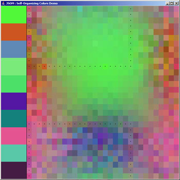 after 15 iterations
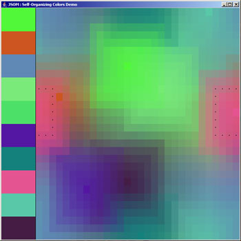
 after 100 iterations
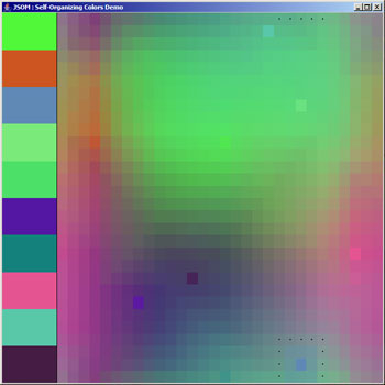
 after 1000 iterations
 after 2000 iterations
Once this happens, the SOM is trained. Assuming we have target values to label each of the nodes in the map, we can then use the SOM as a multi-dimensional lookup table for any color. As a totally useless example, say we train the SOM with 3 colors, red, yellow, and blue, and we will be able to decide for ANY color which of these primary colors it is closest to. A more useful example might to train a SOM to recognize the handwritten letters of the alphabet.
The SOM is often presented as a lattice of hexagons. Here is an example of a hexagonal SOM after about 40 iterations
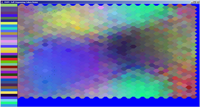 hexagonal lattice
The following java program is an executable .jar file which can be downloaded and executed simply by double clicking on it, or by typing 'java -jar JSom.jar'
Obviously this is not the most aesthetic illustration. But it served my purposes of understanding in detail the process of creating a SOM. In the future I will extend this software as a general purpose Java implemetaion of the original SOM-PAK software, as well as include additional visualizations and examples.