Visualizing the "concrete" Attributes of a Dataset

There are 3 prominate types of data manipulation/visualization:

• Modelling
• Scalar
• Vector

_________________________________________________________________________________________

Modelling:

Modelling includes manipulation of dataset geometry as well as creating polygon objects for the visualization image.

• texture coordinates
• axes
• labels
• objects to provide context

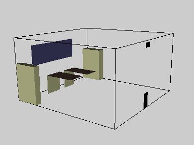
In example 11, the location of tables, filing cabinets, bookshelves, windows, and air inlets and outlets are modelled.

_________________________________________________________________________________________

Scalars:

Scalar values are those that have only magnitude (including sign). Some basic forms of visualizing scalar data in 3D space include:

• contouring (aka isosurfaces)
• colormapping
- requires geometry onto which to put the colors:
- plane
- spheres at each cell or cell corner
- isosurface

•multitude of colormap selections
• volume rendering (covered later) is a special rendering technique that does colormapping
• height/terrain map

Typical scalar values include, density, water vapor, pressure, temperature. However, there are also ways to create scalar values from other data:

• height (z-value) of a vertex
• magnitude of a vector
• dot product of a vector with a surface's normal
• number of visits of a moving particle to a region of space

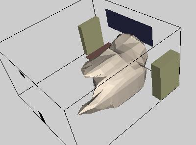
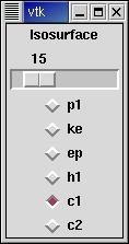
In example 12, an isosurface is generated from the selected scalar value (all the scalars in this example are preexisting within the data file).

In example 13, a cutting plane visualizes a slice of the chosen scalar value.

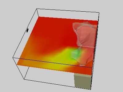
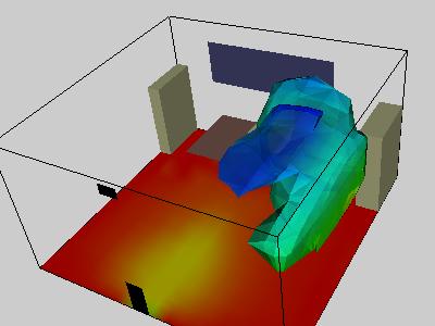
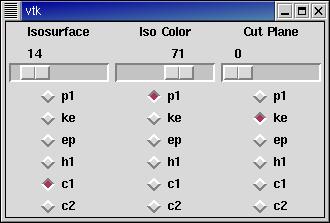
In example 14, the isosurface can be colored by one value with different scalars affecting the shape of the surface and color of the plane. Also, transparency control now exists for the isosurface to allow the user to determine the optimal value.

___________________________________________________________________________________________________________________________

Vectors

Vector values have magnitude and 3D direction components. Some basic forms of visualizing vector data in 3D space include:

• glyphs (including lines and arrows)
- basically an expanded representation of a line
- may also have a representation of direction
- need to watch out for clutter
- need to be wary of scale misrepresentations
• shape warping
• displacement plot
• flow

Typical vector values include:

• fluid flow (eg. wind, water, cosmic matter)
• simple stress forces
• magnetic flux

Vector fields can be created by calculating the gradient of any 3D scalar field.

• change in height
• change in pressure

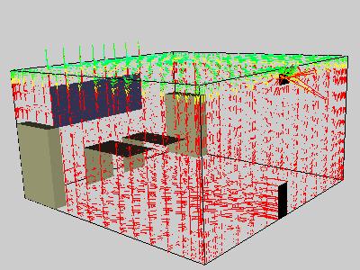
In example 15, the vtkHedgeHog module is used to create simple two segment arrows from each vertex. Pattens can be seen when lines are condensed, but it's a bit hard to see the lines when zooming in.

In example 16, the vtkGlyph3D module is used to put a 3D geometry at each vertex. The cone is a good simple geometry to use for this.

____________________________________________________________________________________________________________________________________